|
(21) |
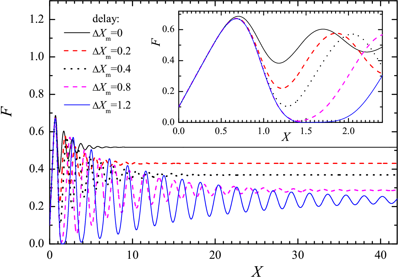 |
Figure 6: The dependences F(X) for different delay times. The distribution Pc(x) is Gaussian with xs= 1 and σs= 0.2, the initial distribution Qini(x) is Gaussian with xini= 0.1 and σini= 0.025. |
Now let us take into account the aging of
contacts (see also
![]() and
and
![]() for more details). Experiments as well as MD simulations indicate that the static
friction force grows with the time of stationary contact (the waiting time tw, i.e., the duration of static contact prior to sliding). Thus, if the newborn
contacts are characterized by a distribution Pci(x) with the average xsi and
dispersion σsi , then
typically xs grows while σs decreases with time, and
at t → ∞ the distribution
Pc(x, t) approaches a distribution Pcf(x) with xsf > xsi and σsf < σsi. If we assume that the evolution of
Pc(x) corresponds to a stochastic process, then it should be described by the
Smoluchowsky equation
for more details). Experiments as well as MD simulations indicate that the static
friction force grows with the time of stationary contact (the waiting time tw, i.e., the duration of static contact prior to sliding). Thus, if the newborn
contacts are characterized by a distribution Pci(x) with the average xsi and
dispersion σsi , then
typically xs grows while σs decreases with time, and
at t → ∞ the distribution
Pc(x, t) approaches a distribution Pcf(x) with xsf > xsi and σsf < σsi. If we assume that the evolution of
Pc(x) corresponds to a stochastic process, then it should be described by the
Smoluchowsky equation
|
(22) |
the "diffusion" parameter D describes the rate of aging, B(x) = dU(x)/dx, and the "potential" U(x) is defined by the final distribution, Pcf (x) ∝ exp[−U(x)] so that
|
(23) |
Then, the equation ∂Pc/∂t = DLxPc naturally leads to the growth of the average static threshold from xsi to xsf with the time of stationary contact, as widely assumed in earthquakelike models of friction (e.g., see Eq.(Fs) in previous Chapter). At the same time, the contacts continuously break and reborn when the substrate moves, as described by third and forth terms in Eq.(6). Combining both the processes together, we come to the system of three equations:
|
where DX
|
|
Figure 7: Evolution of Pc(x) due to two concurrent processes: the first is the aging of asperities from the initial (fresh) distribution Pci(x) (Gaussian with xsi= 0.5 and σsi= 0.05) to the final distribution Pcf (x) (Gaussian with xsf = 1 and σsf = 0.02), and the second is the break/reborn process. DX ≡ D/v = 5×10
|
In the result, the friction force F now depends on the sliding velocity as shown in Fig.8.
|
|
Figure 8:
(a) The final
distribution Qs(x) for five
values of the parameter DX
(b) The corresponding distributions Pc(x); larger circles show the initial distribution Pci(x) (red) and the final distribution Pcf (x) (blue).
Inset demonstrates the dependence of the kinetic friction force F in the steady state on the driving velocity v. Here ‹ki› = 1, Pci(x) is Gaussian with xsi= 0.5 and σsi= 0.1, and Pcf (x) is Gaussian with xsf = 1 and σsf = 0.01.
Note: because typically xsi< xsf , the force F decreases when v grows, so that dF(v)/dv < 0; that may lead to instability of the smooth sliding regime
|
If the sliding block is not rigid, K < ∞, the system
will demonstrate either stick-slip or smooth sliding depending on the distribution
Pc(x); in this case the effect of
contact's aging must lead to the transition from stick-slip to smooth sliding
with the increase of sliding velocity (for details see
![]() and
and
![]() ).
).
Note: in the case of contact of rough surfaces, the physical mechanisms of contact aging, according to Baumberger and Caroli (2006), are the following: the first (and more important) mechanism is due to geometrical aging, or the increase of contact area at the asperity, and the second, due to structural aging, or restructuring of the contact. The value of the parameter D in Eqs.(24) may be estimated from experiments which show that in most cases the average static threshold μs= Fs/Fload grows logarithmically with the waiting time tw, dμs/d(ln tw) ≈10-2.
|
(25) |
|
(26) |
|
(27) |
|
(28) |
|
(29) |
and the function H(x) in Eq.(27) is determined by
|
(30) |
On the other hand, for "stiff", or "strong" contacts, when ΔE(0; xs) >> kBT, we have to substitute in Eq.(28) for the activation energy the expression ΔE(x; xs) = ΔE(0; xs) (1−x/xs)3/2, and also to renormalize the prefactor ω, ω → ω (1−x/xs)1/2. In this case the function H(x) is to be calculated as
|
(31) |
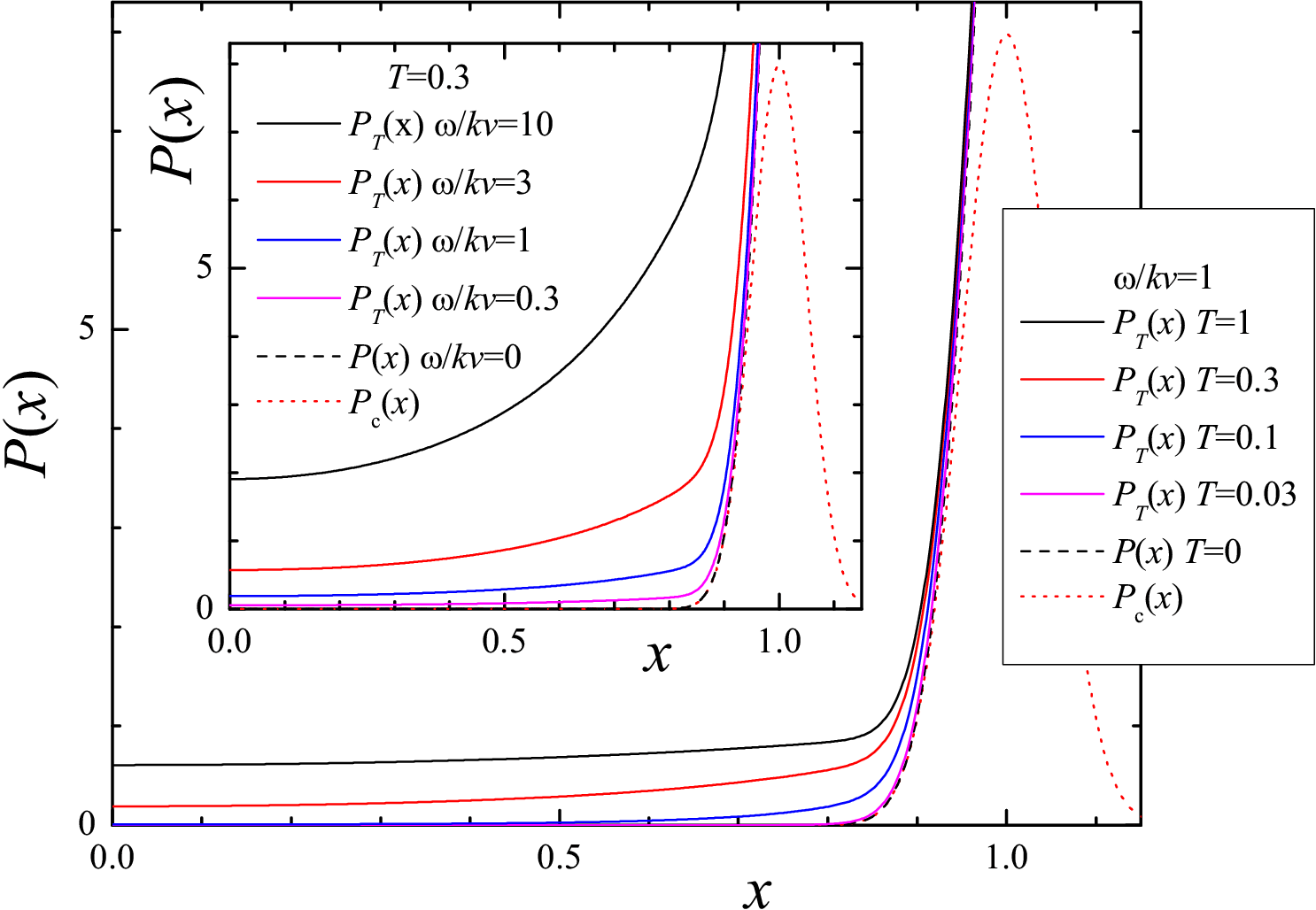
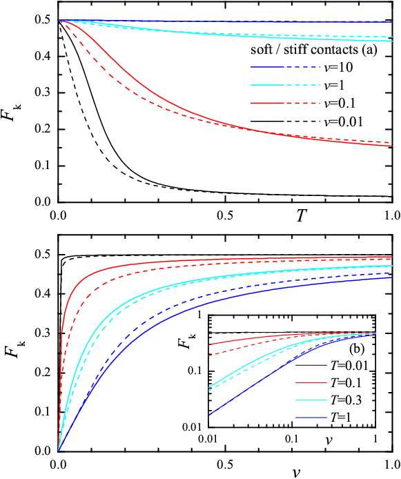
The contribution (30) or (31) to the rate PT(x) leads to appearance of a low-x tail. Its height grows with temperature as well as with decreasing of the driving velocity v as demonstrated in Fig.9. The increase of temperature leads to a shift of the distribution Q(x) to lower values, so that the friction force decreases when T grows. The effect is the larger, the lower is the sliding velocity as shown in Fig.10. In the limit v → 0, all contacts will finally break if T > 0, so that Qs(x) → δ(x) and Fk→ 0; in this limit we have "smooth sliding" corresponded to creep motion of contacts.
 |
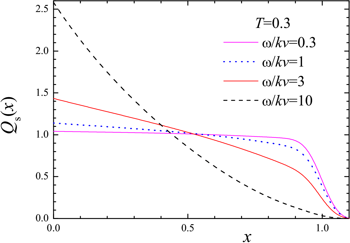 |
| Figure 9: The rate PT(x) for soft contacts at different temperatures T = 0 to 1 for a fixed velocity ω/kv = 1, and (inset) at different velocities, ω/kv = 0 to 10, for a fixed temperature T = 0.3. Dotted curve shows the distribution Pc(x) (Gaussian with xs= 1 and σs= 0.05). | Figure 10: The steady-state distribution Qs(x) for T = 0.3 and different velocities (ω/kv = 0.3, 1, 3 and 10) for soft contacts. The distribution Pc(x) is Gaussian with xs= 1 and σs= 0.05. |
 |
 |
|
Figure 11: (a) Dependence of the kinetic friction force Fk in the steady state on temperature for different velocities v = 0.01, 0.1, 1 and 10. (b) Fk(v) for different temperatures T = 0.01, 0.1, 0.3 and 1; inset shows the same in log-log scale. Solid curves are for soft contacts, and broken curves, for stiff contacts. The distribution Pc(x) is Gaussian with xs= 1 and σ = 0.05; ω/k = 1. |
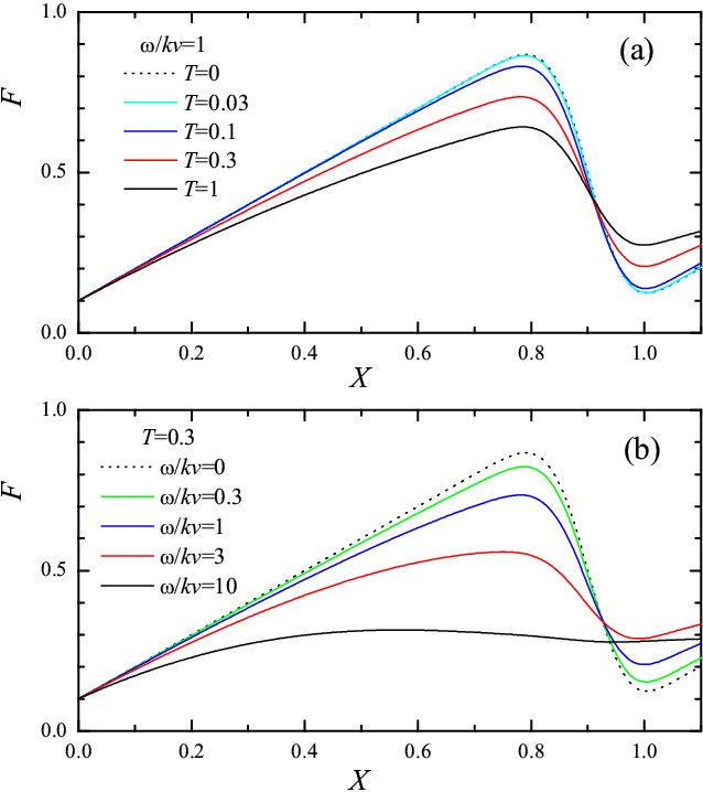
Figure 12: The dependences F(X) for short X. (a) F(X) for different temperatures T = 0, 0.03, 0.1, 0.3 and 1 at the fixed velocity ω/kv = 1; (b) F(X) for different velocities v, ω/kv = 0, 0.3, 1, 3 and 10 at the fixed temperature T = 0.3. |
Nonzero temperature
influences on the dynamics of approaching to the steady state (see Figs.12 and
13). The higher is temperature
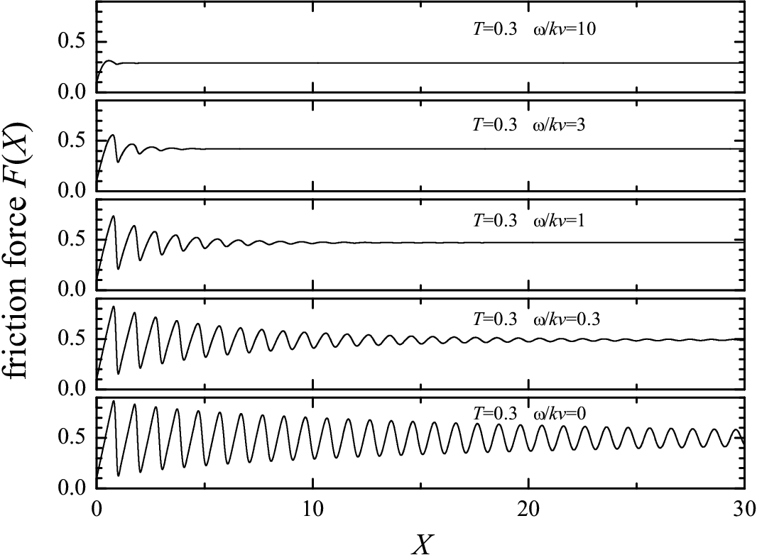
and/or the lower is velocity, the lower is the static friction force Fs determined by the first maximum of F(X), and the faster F(X) approaches to the steady-state smooth sliding. Also it is important to consider the
first cycle of the F(X) dependence, which defines the
lowest value of F'(X).
The higher is
temperature, the lower is the extremum of F'(X) (see
Fig.12a),
so that the larger is the interval of model parameters where the smooth sliding
regime operates. At the same time, the higher is driving velocity (Fig.12b),
the smaller is the lowest value of F'(X),
so that the narrower is the interval of model parameters where the smooth
sliding regime operates (also see
![]() ). Thus, we come to a surprising conclusion that at
T > 0
the decreasing of pulling velocity may lead to the transition from stick-slip to
smooth sliding, i.e., the scenario just opposite to the conventional one (in
fact, stick-slip shoud exist for an interval of driving velocities and disappear
low lower and higher velocities, see
). Thus, we come to a surprising conclusion that at
T > 0
the decreasing of pulling velocity may lead to the transition from stick-slip to
smooth sliding, i.e., the scenario just opposite to the conventional one (in
fact, stick-slip shoud exist for an interval of driving velocities and disappear
low lower and higher velocities, see
![]() ).
).
|
Figure 13: The dependences F(X) for T = 0.3 at different driving velocities
v,
ω/kv = 0,
0.3, 1, 3 and 10.
The distribution Pc(x) is Gaussian with xs= 1 and σs= 0.05, the initial distribution Qini(x) is Gaussian with xini= 0.1 and σini= 0.025. |
The described behavior of Fk on T and v qualitatively agrees with the tip-based experiments. Surprisingly, the dependences obtained within the ME approach, perfectly agree with the experimental ones for a "model" tribological system, where the kinetic friction of the driven lattice of quantized magnetic vortexes in high-temperature cuprate superconductors was studied (e.g., compare inset of Fig.11b with Fig.3 of Maeda et.al. Int.J.Mod.Phys. B 19 (2005) 463).
Last updated on April 19, 2014 by O.Braun. Translated from LATEX by TTH