Earthquakes

We introduce a simple model of earthquakes, inspired by the spring-block models, but describing contacts at a meso-scale. A single contact point synthesizes many rock contacts so that these "macro-contacts" can have an internal dynamics, described by a stochastic process, that leads to an evolution of their breaking threshold. This aging process leads to the Gutenberg-Richter law, which relates the probability of occurrence of earthquakes to their magnitude. An analytical approach based on the master equation technique is used to determine the range of magnitudes in which this law applies. Then, incorporating the elasticity of the sliding plates, we reproduce also the Omori aftershock law. Thus, the simultaneous incorporation of aging of contacts in the sliding interface and of elasticity of the sliding plates constitute the minimal ingredients to account for both laws, the Gutenberg-Richter law and the Omori aftershock law, within the same frictional model.

Gutenberg-Richter law

The hyperbolic law (1), in contrast to the exponential decay typical for most phenomena in physics, indicates a long-lived nature of the EQ activity or some self-organized phenomenon. The first physical model of EQs was proposed by Burridge and Knopoff − the well known BK spring-block model − and further developed in many studies. In these models, two plates are coupled by a set of contacts which deform when the plates move relatively to one another. The contacts are frictional, i.e., they behave as elastic springs as long as their stresses are below some threshold  σ_s and break and re-attach in a less-stressed state when the threshold is exceeded. The EQ amplitude A is typically associated with the number of broken contacts s at an event. Typically these models demonstrate a GR-like power-law behavior,

A more realistic model is obtained if each contact is characterized by its own threshold  f_si, with a continuous distribution P_c(f_si). Typically one assumes that P_c(f_si) is Gaussian with an average  f_s and a standard deviation δf_s. These models may also exhibit a power law (4), but now s_m is determined by model parameters and remains finite when the system size increases. However the interval of M values where the power law is valid in simulations is typically ΔM ~ 2, i.e., much smaller than that observed in real EQs, where ΔM > 6. One possible extension of these block-springs models is to incorporate a slow relaxation of the stress at contacts to account for their plastic deformation.

On the other hand, EQ-like models appeared rather successful in recent studies of friction. Moreover, kinetics of the EQ model may be reduced to a master equation (ME) which allows an analytical study. This approach describes, with some generalizations, the temperature effects and may incorporate aging of contacts (frictional strengthening of the interface due to, e.g., growth of the contacts' sizes, or their reconstruction, chemical "cementation", etc.).

The ME approach naturally introduces a concept of "macrocontacts" (λ-contacts). Such macrocontacts have properties which are much richer than individual ones, and may depend on time as the dynamics of individual contacts modify their collective properties. This introduces the idea that contacts could have time-dependent properties, which would be useful at the scale of earthquakes too. In this context, considering the frictional contacts as "static" ones having fixed parameters such as thresholds and stiffness can be questioned. This may be acceptable for the frictional interface where the plates move with a speed up to m/s, but is unlikely to be true for EQs where the typical velocity of a tectonic plate is v ~ 30 mm/year ≈ 3×10^–9 m/s. Here we propose a EQ-like model with "living" λ-contacts, where the contact parameters are not fixed but evolve with time from event to event. The contacts in our model actually describe the interaction of two tectonic plates at a rather large scale, i.e. must be regarded as macrocontacts. An earthquake can be the breaking of a single of these macro-contacts, although, if they are interacting it may also involve several of them. We show that, if one describes the aging of those contacts as an independent time-dependent statistical process, this process can be responsible for a Gutenberg-Richter law for the statistics of the events. We then show how the master equation approach applied to this extended model can be used to evaluate the largest magnitude for which the model can lead to the GR law.
 

Model. We consider a tectonic plate that slides with a velocity v over another plate, called the base, which is taken as the reference point assumed to be fixed. The two plates are coupled by an array of contacts, which should be viewed as describing a larger scale than the simple contacts in BK-type models because they synthesize in a single connection the many interactions that occur between the rocks in a region of a fault. To give an order of magnitude, one can consider that a "contact" represents the interaction of the two sides of a fault on a scale of a few kilometers, while the actual "micro-contacts" of the rocks take place at a scale which can be of the order of millimeters to meters.

In the spirit of the spring-blocks models, we consider a two-dimensional array of contacts organized in a triangular lattice of size N and lattice spacing a with periodic boundary conditions. Each contact is characterized by a shear force  f_i= k_il_i, where k_i is the contact stiffness and l_i is its stretching. Each contact is also characterized by a threshold value  f_si; the ith contact is elastic until |f_i| < f_si but breaks when the stress exceeds the threshold. We assume that the thresholds  f_si have a continuous distribution P_c(f); the elastic constants k_i also have a continuous distribution which is coupled with the distribution P_c(f) as k_i= k(f_si/f_s)^1/2 (see ). When a contact breaks at  f_i = f_si, it takes a value  f_i~ 0, and a new value for its threshold is assigned. The (rigid) plate moves by ΔX per time step Δt = ΔX/v (in contrast to the cellular automaton algorithm, here we assume that ΔX is fixed), and all contact stretchings get the increment ΔX per time step.

Our numerical algorithm is organized in the following way. At each time step we look for the largest value of  f_i− f_si and, if it is ≥0, the ith contact breaks so that the total force on it (together with the contribution Δf_i due to interaction with the neighboring contacts when it is taken into account) becomes equal to zero, i.e., the contact is restored in the "zero force position". Then, at the same time step, we recalculate all Δf_i values and again look for the largest one, repeating the process until all forces fall below the thresholds that break contacts, and calculate the corresponding drop of the force applied to the sliding plate from the contacts, ΔF_i, at the given time step.

Elasticity of the sliding tectonic plates leads to an interaction between the contacts: when one of the contacts breaks, the shear stress sustained by this contact must be redistributed among the neighboring contacts and may even cause an avalanche of contacts breaking. To incorporate this effect, we assume that because of the elastic interaction between the contacts i and j, the forces acting on these contacts have to be corrected as f_i→ f_i− Δf_ij and f_j→ f_j + Δf_ij, where Δf_ij= k_ij(l_j− l_i) in the linear approximation. For example, let at t=0 the contacts be relaxed, l_i(0) = l_j(0) = 0, and then, due to plate motion, all stretchings grow together, so that still Δf_ij= 0. Then, let at some moment t the jth contact breaks, l_j(t) → 0, while the ith contact is still stretched, l_i(t) > 0, so that Δf_ij(t) = − k_ijl_i(t) < 0. Therefore, when the jth contact breaks, the force on the ith contact increases. To incorporate the interaction between the contacts in our model, we assume that the stretching of the given (ith) contact has an additional contribution Δf_i= Σ_j'k_ij(l_j− l_i), where the sum is over the neighboring contacts inside some circle of the radius r_c (in simulation we used r_c= 3a), and k_ij∝ r_ij^–3; we put k_ij= κk(a/r_ij)³, where the dimensionless parameter κ (which is an analog of the parameter α in the OFC model ) characterizes the strength of interaction (a more rigorous model is introduced below, where the Omori law is discussed).

Finally, we can also incorporate a slow relaxation of contacts (e.g., because of transient material creep) in order to allow for spatio-temporal correlations between the events. We assume that at every time step (after checking/breaking the contacts), all thresholds are "relaxed" according to a "diffusion" law (r is the 2D vector in the interface)

Aging of contacts. While the other features of our model are similar to earlier studies, the description of aging is the important new feature of the approach. Besides the dynamics of the cellular automaton, we introduce a second dynamics for the properties of the contacts, which is particularly important because, as discussed above, in this model the contacts synthesize many actual rock contacts and can therefore have their own dynamics. Newborn contacts emerge with a threshold f_si~ 0, but then the threshold value should grow with time due to contact aging, i.e., the plastic deformations at the level of the rock contacts or the slow formation of chemical bonds, due for instance to the effect of the ground water. Because this evolution is actually due to local changes occurring at the many individual rock contacts, it can be represented as a stochastic process described by the simplest stochastic equation df_si= K(f_si) dt + G dw  with  <dw > = 0  and  <dw dw> = dt, where K(f) and G are the so-called drift and stochastic forces correspondingly. Alternatively, this process is described by the Langevin equation

Our main assumption is that the drift force is given by the expression

K(f) = (fs/τ0) β2 1 − f /fs 1 + ε (f /fs)2  ,

(7)

while the amplitude of the stochastic force is equal to

G = β δ fs √ 2/τ0  ,

(8)

where β and ε are two dimensionless parameters. With this choice, the stationary solution P_c0(f) of the FPE corresponds to the Gaussian distribution P_c0(f) = (2π)^–1/2(δf_s)^–1exp[−(1/2)(1 − f /f_s)²/δ²] in the case of ε=0, while for ε>0 the distribution of thresholds has a power tail, P_c0(f) ∝ f ^–1/εδ2 for  f >> f_s. For εδ² < 0.5 the average threshold tends to saturate to a finite value while for εδ² > 0.5 it keeps growing. Thus, the dimensionless parameter ε determines the deviation of the distribution of thresholds from a Gaussian one, while the parameter β corresponds to the rate of aging, which should be compared with the driving velocity set to v = 1.

Simulation. Four parameters of our model may be fixed without loss of generality; we put a = 1, v = 1, f_s= 1 and k = 1. Then, the natural unit of length is a₀= f_s/k = 1 and the natural time unit is τ₀= a₀/v = 1. The parameter δ = δf_s/f_s describes the thresholds dispersion; in what follows we put δ=1. Thus, our model is characterized by four dimensionless parameters:

• ε describes a deviation of the threshold distribution P_c(f) from the Gaussian one,
   
• β describes the rate of aging (in our units the limit v → 0 corresponds to β → ∞),
   
• κ describes the strength of interaction, and
   
• D = D/(a²/τ₀) describes the rate of relaxation.

We define the (dimensionless) amplitude of a EQ as the sum of the drops of forces on contacts at every time step, A = Σ_i ΔF_i /f_s. In simulation we typically used the lattice N = 30×34 = 1020 so that M_max~ (2/3) log₁₀N ≈ 2. In the initial state, all contacts are relaxed,  f_i= 0. The simulation time was t_max= 10³τ₀ or longer; the first ~10% of data were discarded to reach the steady state. The displacement step was ΔX = 10^–4a₀, but we checked how a change of ΔX may disturb the results. The results are presented in Figs.1 and 2.

Figure 1: The distributions P(M) for κ = 0, D = 0 and N = 1020: (a) for β = 10 and different values of ε  (tmax= 103), and (b) for ε = 0.5 and different values of β  (tmax= 104). Line shows the GR power law with b = 1.

Figure 1b shows that the power-law interval ΔM increases with β: the slower the plate moves, the larger is the interval of EQ magnitudes where the GR law operates.

Figure 2: The distributions P(M) for ε = 0.5, β = 100 and different values of κ and D (N = 1020, tmax= 5×103).   Line shows the GR power law with b = 1.

Figure 2 demonstrates the role of interaction (κ > 0) and relaxation (D > 0). Interactions and relaxation of the contacts have qualitatively similar effects, they tend to kill large EQs while significantly increase the number of small events, which exceeds the number expected from the GR law. For earthquakes this would correspond to events that occur in several places quasi-simultaneously, a small earthquake in one place (breaking of a contact) leading to another small one nearby, triggered by the interaction. In other words, the interactions tends to favor the relaxation of the tensions before a very large event has time to build up.

Master equation. The results plotted in Fig.1 show that, in the presence of aging, this model is able to exhibit a GR law for the statistics of the events. As discussed in the introduction, the question posed by all simplified models of earthquakes is the range of validity of this law, which is generally found to be limited, not only by the size of the model system but rather by fundamental limits of the model. To examine this aspect for our model with aging, let us consider the simplest model which gives the GR law, i.e. ignore the interaction between the contacts as well as their relaxation, κ = D = 0, and study it with the ME approach.

Let P_cx(x) be the normalized probability distribution of values of the stretching thresholds x_si at which contacts break; it is coupled with the distribution of threshold forces by the relationship P_cx(x)dx = P_c(f)df.  When κ=D=0, the earthquake event corresponds to the breaking of a single contact, thus P_cx(x) determines the statistics of earthquakes. To describe the evolution of the model, we introduce the distribution Q(x; X) of the stretchings x_i when the bottom of the sliding plate is at a position X. The stationary solution Q_s(x) of the ME can be found analytically.

However, this formal solution is not yet the full solution of the problem because P_cx(x) is unknown − it should result from the aging of the contacts. Above we introduced Eq.(6) which tells us how the distribution of the thresholds evolves under the effect of aging alone. This equation may be rewritten as

Thus, we come to the set of equations, Eq.(19) plus Eqs.(4−6) from the ME approach. For the steady-state regime in the case of R(x) = δ(x), Eq.(19) reduces to

Discussion. When we discuss the GR law in terms of P_cx(x) we assume that an earthquake is associated to the breaking of a single contact, i.e. we put A = f. This is legitimate because we have considered the case κ=0, i.e. we do not take into account the interaction between the macrocontacts. Therefore a breaking does not induce another breaking in its vicinity. However, this does not mean that, in our algorithm where the motion of the plates occurs in steps ΔX, two events cannot occur fortuitously at the same step. In the cellular automaton algorithm, where every EQ event is treated separately (this corresponds to the MD algorithm in the limit ΔX → 0), the EQ distribution is equal to

However, in the MD algorithm with a finite step ΔX, there is a nonzero probability that two events may occur during the same step; the distribution of such events is P₂(f) ∝ (P₁⊗P₁)(f), and so on for the occurrence of several events during the same step. This could affect the statistics that we measure in the simulation. However this effect is mostly likely to occur for distributions P_cx(x) which are highly peaked and tend to concentrate the events. For the case of interest for earthquakes, where the distribution has a tail at large x, the probability of quasi-simultaneous occurrence of events is low, and the simulation determines P_cx(x) with a good accuracy when ΔX is small enough. We have tested this by performing simulations with different steps. The step ΔX = 10^–4 has been used for the results presented in figures above. It corresponds to a time interval Δt = ΔX/v. With v=1 and events observed with a time interval of a few units in the calculations, if we consider that a real earthquake has a duration of the order of a minute, it sets the time scale for the value Δt = 10^–4 in the calculations. Events separated by a few time units in the calculation are separated by a few weeks in actual time, which is a realistic scale validating the choice ΔX = 10^–4.

The main result of this work is that the GR law for earthquakes emerges because of the aging of contacts. This is possible because a "contact" is actually describing many rock interactions and has its own dynamics. Of course, the model could be completed in many ways to approach more realistic situations. We showed here that interaction and relaxation of the contacts tend to reduce the domain in which the GR law applies, essentially because they tend to facilitate the occurrence of small events that relax the system. One thing that is missing in such a description is the elasticity of the plates; as will be shown in next section, it is responsible for the Omori law for aftershocks .

Equation (24) shows that the largest earthquake above which one could expect the GR law to break down is determined by the velocity v of the moving tectonic plate and the parameter β which measures the rate of aging. Therefore, as these quantities can be expected to be roughly constant for given tectonic plates, statistics on one region could be used to infer the risks in another region belonging to the same plate.

The process describing the aging of the contacts needs further investigations as it is presently largely arbitrary. We use a stochastic process that goes to a Gaussian distribution in one limit and a power law in another, but how the aging process can be generated by the dynamics of "macro-contacts" is still open.

Published in: O.M. Braun and M. Peyrard, Phys. Rev. E 87 (2013) 032808 "Role of aging in a minimal model of earthquakes"

Omori law

The second well known, empirically established law of planetary scale friction (i.e., seismology) is the Omori law. It describes the rate of aftershocks (in excess of the background value) at time t after the main event, n(t) = K_O/(τ_c+ t)^p, where K_O is proportional to the magnitude M of the main shock, τ_c has a typical average value of about 7 hours, and p ≈ 1 (or more generally p = 0.7−1.5). A similar behavior (with Δt → −Δt) was also reported for foreshocks. Note that both the GR law and the Omori law were established through a statistical analysis of observed EQs. Although widely addressed and discussed theoretically, a generally accepted frictional model whose solution simultaneously accounts for both laws is still lacking.

Model. As above, we assume two plates, the top plate (the slider) and the bottom plate (the base), coupled by a multiplicity of frictional micro-contacts. To incorporate the elasticity of the slider, we use the recently developed multiscale theory of the frictional interface, where the sliding proceeds through creation and propagation of self-healing cracks. Recall that elastic theory introduces a characteristic distance λ_c known as the elastic correlation length, below which the frictional interface may be considered as rigid. Roughly it may be estimated as λ_c< or ~ a_c²E/k_c, where a_c is an average distance between the micro-contacts, E is the Young modulus of the slider, and k_c is the elastic constant of an individual micro-contact. A set of N_c= λ_c²/a_c² micro-contacts within the area λ_c² constitutes an effective macro-contact (the λ-contact) with elastic constant k = N_ck_c. The macro-contacts (simply called contacts from now on) are elastically coupled through the deformation of the slider's bulk. If we denote by u_i the displacement of the point on the slider to which the ith contact is attached, then the elastic energy stored between two nearest neighboring contacts i and j in a non-uniformly deformed slider may formally be written as (1/2)K (u_i− u_j)², where K is the slider rigidity defined below. We elaborate here the simplest one-dimensional (1D) version of the model, where the contacts constitute a regular chain of length L=Na with the spacing a = λ_c as shown schematically in figure . The base (the bottom block BB) is assumed to be rigid, whereas the top plate (the top block TB, the slider) of length L is elastic with rigidity K = EHW/L, where H is an effective slider height (thickness) and W its width (in our 1D model we must set W = λ_c). Let us formally split the TB into N = L/a rigid blocks of size a = λ_c; these blocks are coupled by springs of elastic constant

KL = NK = EH = E λc (H / λc)

(O1)

(note that H >> λ_c must hold for the correlation length λ_c to be defined). We describe the contact between the TB and BB in the form of an interface layer (IL) of thickness H_c~ λ_c, consisting of N contacts coupled by springs with elastic constant

K = EcHc ≈ E λc .

(O2)

The IL and TB are coupled elastically with a transverse rigidity K_T= [E/2(1+ν_P)](LW/H) (here ν_P is the slider Poisson ratio) which we model by N springs of elastic constant

KT =  KT N  =  E λc 2(1 + νP)   λc H  .

(O3)

Finally, the IL is coupled "frictionally" with the top surface of the BB − each contact between the two plates is elastic with stiffness constant k as long as the local shear stress in the IL is below the threshold. The interface is stiff if k ~ K and soft when k << K; here we concentrate on the latter case.

Now, if a lateral pushing force is applied, for example, to the left-hand side of the slider as shown in the figure, the stress is transmitted to each contact due to the elasticity of the slider. In this case the interface dynamics starts by relaxation of the leftmost contact which initiates the sliding. This causes an extra stress on the neighboring contacts, which tend to slide too, and the domino of sliding events propagates as a solitary wave, extending the relaxed domain, until the stress at some contact will fall below the threshold. Such a self-healing crack propagates for some characteristic length Λ − leaving a relaxed stress behind its passage, but raising the interface shear stress ahead of the crack (see ). The value of Λ may be estimated analytically; roughly Λ/a is proportional to H/λ_c as well as to k/K.

Besides elasticity, we also incorporate into the model the aging of contacts as was described above.

Simulation. In simulations we used a chain of N = 901 macro-contacts with periodic boundary condition. Four parameters of our model may be fixed without loss of generality: a = 1 (the length unit), K = 1, m = 1 (mass of the macro-contact), and F_s= 1. Then, the characteristic frequency is ω₀= (K/m)^1/2= 1, so that the unit of time is τ₀= 2π/ω₀= 2π. For the elastic slider we used N_L= H/λ_c= 100 so that K_L= N_LK and K_T= K/(2.6N_L). We took ν_P=0.3 for the Poisson ratio, and M = N_Lm for the mass of TB blocks. The top layer of the slider is driven with the constant velocity v = 0.01 through springs attached to the TB blocks, each with the elastic constant K_d = 0.03K. In simulation, the contacts elastic constant is k = 0.03K and the thresholds dispersion parameter δF_s= 0.1F_s; that yields a characteristic distance for self-healing crack propagation Λ ~ 100a. A contact aging parameter ε = 75 yields a GR distribution with b ≈ 1; a reasonable rate of aging is chosen as β = 1. The newborn contacts emerge with a threshold F_si taken from the Gaussian distribution with average F_{s, nb}= 0.01F_s and deviation δF_{s, nb}= F_{s, nb}. In the initial state, all contacts are relaxed, F_i= 0, and all thresholds correspond to newborn contacts. Then, the equations of motion for all blocks (with a viscous damping coefficient η = 1) together with the Langevin equations for contact breaking thresholds are solved with a time step Δt = 0.01. The total simulation time required is t_max= 2×10⁷. In contrast to the cellular automaton algorithm typically used in simulation of the Burridge-Knopoff model, in the present work we use, following Carlson and Langer (1989), the algorithm with a fixed time step Δt. Although in this case it may occur more than one contact breaking event (which corresponds to an earthquake in our model with "living" macro-contacts) per one time step, this does not disturb our main results (see discussion above). We define the (dimensionless) quake amplitude as the sum of force drops on contacts at every time step, A(t) = Σ_i ΔF_i/F_s, and the rate of shocks n(t) as the number of shocks per one time step (regardless of their amplitude).

Figure O2: Time evolution of the system:   (a) the driving force F(t), and   (b) the (global) amplitude of EQs  A(t) versus time.   (c) Statistics of EQ magnitudes presented in (b) (the first 33% of data discarded) showing the Gutenberg-Richter power law behavior; the dashed line corresponds to the exponent b = 1.

The results are presented in Figs.O2 and O3. A typical time sequence of EQ shock sizes is that of Fig.2b. On large time scale, the function A(t) appears stochastic. On a finer scale though (Fig.O3b) one can distinguish separated shock blocks, each with a large main shock followed by aftershocks.

Figure O3: A typical earthquake in the model:   (a) the color map of the EQ amplitude on the (t,x) plane, and   (b) the EQ amplitude  A(t) versus time.

Analysis of results. Now we can analyze the EQ shocks for their characteristics, distribution and correlations in space and time. To do that efficiently, we first remove from the analysis the small "background" EQs with amplitudes below some level − we retain only A  >  2<A(t)> (broken red line in Figs.O2b and O3b). Next, we single out the main EQs (MEQs) above some level A_MEQ; we took here A_MEQ= 0.2A_max (red line in Figs.O2b and O3b). We also used a rescaling procedure to distinguish from one another MEQs that may occur too close: namely, if n_MEQ is the total number of MEQs, call σ=S/n_MEQ the average area occupied by a single MEQ on the (t,x) plane, with S=t_maxL. We then rescale the time coordinate t → τ=t/α with α=σ/λ², where λ is some distance chosen in such a way that the distribution of MEQs on the (τ,x) plane becomes isotropic (λ≈235 for the parameters used in Fig.O2). We can now scan all MEQ coordinates on the (τ,x) plane and, if the distance ρ_ij= [(τ_i− τ_j)²+ (x_i− x_j)²]^1/2 between two MEQs i and j is smaller than some value ρ_cut (we chose ρ_cut= 0.75λ), then only the larger of these two MEQs remains as the MEQ, while the lower one is removed from the list of MEQs.

With this protocol we have obtained a set of well separated MEQs isotropically occupying the (τ,x) plane, and we may calculate the temporal and spatial distribution of all earthquakes within some area around every MEQ − we count the EQs separated from the corresponding MEQ by less than ρ₀= ρ_cut/3. Then we collapse all data together, designating τ=0 for every main shock and normalizing shocks amplitudes on the corresponding main shock value.

Figure O4: Foreshocks and aftershocks statistics: the rate of fore- and aftershocks n(τ) (filled circles) and the shock amplitudes A(τ) (open diamonds) relative the corresponding main shock. The curves demonstrate the Omori law.

The EQ distribution − our main result − is presented in Fig.O4: one can clearly see that the aftershocks follow the Omori law. The spatial correlation between the shocks decays exponentially in our 1D model unlike real earthquakes, where the aftershock amplitude decays power-law with distance owing to 3D elasticity; since the origin of that discrepancy is so very clear, it does not worry us. Foreshocks are also observed in simulation, typically with a smaller value of the lag time τ_c.

Foreshocks

Introduction. While two main seismological laws, the Gutenberg-Richter (GR) law for the magnitude distribution of earthquakes and the Omori law for the time evolution of the frequency of aftershocks, are well established empirically and even may be justified theoretically, our knowledge about foreshocks is still limited. If a clear pattern could be distinguished in the foreshock activity it might provide an early warning for earthquakes, but we are still far from this stage. Many earthquakes are preceded by foreshocks, but their frequency can nevertheless vary widely depending on the type of earthquake. Moreover, some earthquakes are preceded by an unexpected calm period, lasting for several hours or more. It is such a period of quiescence, viewed as a characteristic feature of the imminence of the main shock that allowed the only successful prediction of an earthquake, which saved a large number of lives in China in 1975.

Although the mechanisms that generate foreshocks are still under discussion, the existence of some activity before a major earthquake (MEQ) does not seem surprising. However, the fact that a quiescence period could be a characteristic announcement of a MEQ looks more surprising. In what follows we propose a generic mechanism related to the distribution of the threshold P_c (f_si) for the breaking of the contacts along a fault and illustrate it by simulations of the generalized Burridge and Knopoff (BK) spring-block model. Namely, if P_c(f_si) is one-peaked, e.g., Gaussian with the center at f_s and a standard deviation Δf_s, then the total frictional force on N contacts, F = ∑_i=1^N f_i linearly increases with the slider displacement X until the contact forces reach values f_i ~ f_s - Δf_s. Then some contacts start to break, one by one, giving rise to small earthquakes. The growth of F(X) slows down and turns into a decay for larger values of X, and under certain conditions an elastic instability may occur. The top block slides for a distance ΔX >~Δf_s /k while most of the contacts break. This event corresponds to a large earthquake. In this case the earthquake activity increases just before the MEQ; such a scenario is common in natural earthquakes.

However one can expect a scenario which is qualitatively different if the threshold distribution is two-peaked, e.g., when the interface consists of two types of contacts, weak and strong ones with thresholds f_s1 and f_s2 respectively. To see how it works let us consider a simple case. We assume that, when a contact breaks it forms again as a weak contact with probability p or strong contact with probability 1-p, and that the breaking of a contact reduces the friction force by φ. At time t₀ = 0 we start with n₁⁽⁰⁾ = pN weak contacts and n₂⁽⁰⁾ = (1-p)N strong contacts. If the slider moves at velocity v the driving force grows as Nkvt. When it reaches f_s1 at time t₁, all weak contacts break. The friction force drops by φn₁⁽⁰⁾ and the broken contacts reform, leading to n₁⁽¹⁾ = pn₁⁽⁰⁾ = p²N weak contacts and a growing number of strong contacts. The same process can repeat again, leading to an infinite series of foreshocks, while the number of weak contacts decreases as n₁^(j) = p^j+1N. During the time interval t_j - t_j-1 the force has to grow enough to reach f_s1 again after the breaking n₁^(j-1) weak contacts. It requires a time t_j - t_j-1 = φp^jN/(Nkv) so that the total time for the infinite series of foreshocks stays finite ∑(t_j -t_j-1) = (φ/kv)p/(1 - p). After that time only strong contacts persist. As the slider keeps moving, there is a calm period without any foreshock until the strong threshold f_s2 is reached. Then all strong contacts break suddenly, leading to a MEQ.

This picture of contacts with a two-peaked distribution is oversimplified, and would not show all features of real earthquakes, such as the GR law or the Omori law for aftershocks, but it shows how the properties of the contact thresholds are sufficient to lead to seismic quiescence. Let us now consider a more realistic case and investigate its properties.

Model, its parameters and protocol for data analysis. We use the same two-chain model described above, and use dimensionless units, where four model parameters are set to 1, k = 1, λ_c = 1, t₀ = 1 and f_s = 1 so that the other parameters should be compared with those. The IL consists of N=101 λ_c³-cubes, each of mass m = 10^-4, as chosen in our analysis of stick-slip phenomena. The springs between the cubes have the elastic constant K = 100. The UL consists of parallelepipeds of height N_L = 25 (so that their masses are N_L m); for the Poisson ratio we took σ_P = 0.3. With these parameters, the crack propagation distance (where aftershocks are expected) is Λ ~ 30. For the rate of aging we took β = 100, and for the parameter ε we used ε = 2 / Δf_s². With these parameters the statistics of the magnitudes of earthquakes follow the GR law for an interval of magnitudes ΔM ~ 2, which is of course limited by the size of the model. For the dispersion of thresholds we took Δf_s = 0.3.

The initial stretching of the contacts as well as the initial thresholds of the newborn contacts, when they form again after breaking, are taken from a Gaussian distribution with zero mean and dispersion Δf_s. The UL is moved through the springs with elastic constant K_d = 0.5 attached to its top and driven with the velocity v = 0.1. The equations of motion are solved by a Runge-Kutta method with a viscous damping η = 0.3ω₀, where ω₀ = (K/m)^1/2, so that the dynamics of the system is underdamped. With these parameters, the motion of a single λ_c³-block exhibits a stick-slip behavior. The duration of the runs is t_max = 2×10⁶. The first 33% of a trajectory are discarded to allow the system to lose memory from the initial configuration and reach a steady state.

In a simulation we calculate and store the driving force F(t) and the dimensionless quake amplitude defined as the sum of the force drops due to broken contacts at every time step,

A(t) = N Σ i=1  ΔFi (t)/(N fs)  .

The rate of shocks, n(t), is defined as the number of shocks per time unit regardless of their amplitude. The dimensionless earthquake magnitude is defined as

M = 2 3 log10 ( A/A0 ) ,

where A₀ is a constant which defines the magnitude scale.

As for the study of real earthquakes the analysis of foreshocks is delicate because one has to distinguish "main shocks" in the middle of many events, occurring randomly and with a broad range of amplitudes. To be qualified as "foreshocks" events must be related to the main shock both in time and space, and moreover a large foreshock should not be considered as an independent MEQ. In analyzing the results, we used the protocol described above: First we remove small "background" earthquakes with amplitudes below some level from the analysis. We only retain A > 2 <A(t)>. Next, we single out the main shocks above some level A_MEQ. We took here A_MEQ = κA_max, with κ = 0.03. We also used the following rescaling procedure to detect large events which could be related. If n_MEQ is the total number of MEQs in a simulation, let us call σ = S/n_MEQ the average area occupied by a single MEQ in the (t, x) plane, with S = Nλ_ct_max. We then rescale the time coordinate t → τ = t/α with α = σ/λ², where λ ~ Λ is some distance chosen in such a way that the distribution of MEQs on the (τ, x) plane becomes isotropic (λ = 30 and α = 300). In this rescaled space, events which are related to a particular MEQ lie within a circle around this MEQ so that they can be easily identified. We can now scan all MEQ coordinates on the (τ, x) plane and, if the distance ρ_ij = [ (τ_i - τ_j)² + (x_i - x_j)² ]^1/2 between two MEQs i and j is smaller than some value ρ_cut then only the larger of these two MEQs remains as the MEQ, while the lower one is removed from the list of MEQs. We chose ρ_cut = 0.4 λ ~ 0.4 Λ, i.e. to be considered as related to each other two events must not be separated by more than about 0.4 × the average distance along which a crack propagates.

With this protocol we have obtained a set of well separated MEQs isotropically occupying the (τ, x) plane, and we may calculate the temporal and spatial distribution of all earthquakes within some area around each MEQ. We consider that all the events separated from the corresponding MEQ by less than ρ₀ = ρ_cut /3 are related to this particular MEQ. They can be either foreshocks or aftershocks. However we have to make sure that some events that occur before one of the MEQ do not belong to the tail of aftershocks following a violent MEQ which occurred earlier. This is done by examining only MEQs which are separated by a time interval long enough to allow the tail of aftershocks to die out. In practice only MEQs separated by a τ interval greater than 0.4 × the full τ interval that we scan around MEQs are analyzed. This lead us to discard more than 30% of the events that would otherwise qualify as MEQs.

Then we collapse all data together, designating τ = 0 for every main shock and normalizing shocks amplitudes on the corresponding main shock value. We compute n(τ) the number of secondary events (foreshocks or aftershocks) in a given Δτ = 0.0648 interval averaged over all the investigated MEQs as well as the standard deviations of their values for the different MEQs, which provides an estimate of the error bars for n(τ) and gives us an information on the fluctuations of the earthquake activity in a given t interval around a MEQ.

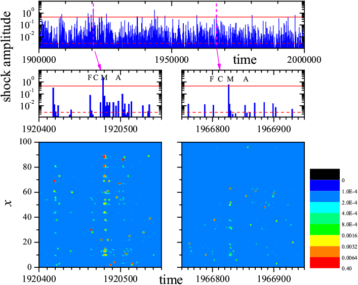
Simulation results. The simulation results are presented in Figs. O5-O6. For the chosen set of parameters, we ran 20 independent calculations using different sets of random numbers, and with the protocol described above we obtained 10.8×10⁶ shocks above the background level and analyzed 7012 main shocks which occurred during the time interval T = 0.67 t _max = 1.34×10⁶ after the first 33% of data were discarded in each simulation. Figure O5 shows the A(t) dependence for the last 5% of the simulation time (top panel) and more detailed pictures at a finer time scale of two typical MEQs (middle panel); the bottom panel of Fig. O5 shows the color maps of the earthquake amplitude.

 Figures O6 presents the main result of the data analysis, the average number of shocks n(τ) in an interval Δτ ( Δτ = 0.0648), versus τ the rescaled time interval from (τ < 0), or after (τ > 0), the corresponding main shock. We show both the mean value n(τ), computed for the 7012 analyzed shocks, and its fluctuations for different MEQs, measured by its standard deviation over all analyzed MEQs. The variation of the fluctuations versus τ are the most interesting. Before the MEQ they are large, and vary widely with τ in the range τ <-0.7, showing a significant and random foreshock activity. Then suddenly they drop to a small value and stay so for the last period before the MEQ, -0.7 <τ < 0. In this range none of the 7012 analyzed MEQs shows any noticeable foreshock activity. As expected, after the MEQ, Fig. O6 shows a large aftershock activity.

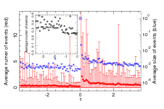Figure O6: Foreshocks and aftershocks statistics in the presence of contact aging (β = 100): the rate of fore- and aftershocks n(τ) (red solid symbols) and their associated standard deviations (red bars), and the shock amplitudes A(τ) (blue squares) relative to the corresponding main shock. The horizontal dash lines show the average magnitudes of the foreshocks and aftershocks. The inset shows the average number of foreshocks n(τ) with a magnified scale. The results plotted on this figure have been obtained from the analysis of 7012 main shocks, collected over 20 independent simulations.

Figure O7 shows that the sharp drop of foreshock activity before large events is clearly due to the aging of the contacts, described by the parameter β. When β is reduced from β = 100 to β = 3 (β = 0 corresponding to no aging at all), all other parameters being preserved, the calm period disappears and a slight increase of activity immediately before the MEQ is even observed. We can also notice that, in the absence of aging, the fluctuations of the foreshock and aftershock activity with time, are much smaller. Similarly the standard deviations of n(τ) between the different main shocks are smaller and almost time-independent.

Figure O7: Same as Fig. O6 with β = 3, i.e. with very little aging of the contacts. In this case the magnitudes of the main events are not as large as in the presence of aging, so that we define the main shocks by AMEQ = κAmax, with κ = 0.4. A set of 1205 MEQs was used to draw this figure.

Relation with the actual scales of earthquakes. To couple our dimensionless units with real ones, we use the following trick: let us calculate the average time between the MEQs as t_rec = T/n_MEQ = 2.8×10³. Then, if we identify this time span with, e.g., 100 days (which is the recurrence time of M > M₀ = 5 earthquakes in Southern California), we obtain the correspondence between time units in our model and in real seismicity:

Discussion. In order to correctly describe various features of earthquakes, the model that we used in this work is more complex than the simplified case that we presented in the introduction, and the probability distribution of the breaking thresholds is not imposed a priori but instead results from the dynamics of the model. Figure O8 shows that the qualitative mechanism for the origin of a calm period that we presented in the introduction is nevertheless also present in this more elaborate case.

While the initial probability distribution of the thresholds for contact breaking P_c(f_si) was a Gaussian, the evolution of the thresholds leads to a very different shape as time evolves. The maximum value of f_si grows, and moreover the distribution tends to split into a large cluster of contacts which break easily (the "weak contacts" of the qualitative model) and a few very strong contacts. The contacts with intermediate thresholds tend to disappear. It is the few strong contacts that prevent the sliding and are responsible for the MEQs when they finally break. The gap between these strong contacts and the many weak contacts is responsible for the calm period. This evolution is mostly governed by the aging of the contacts.

In natural seismicity quiescence is observed in about 40% of events: the frequency of small events is gradually enhanced preceding the main shock, whereas, just before the main shock, it is suppressed in a close vicinity of the epicenter of the upcoming event. In about 60% of natural earthquakes another scenario is observed. Large earthquakes are preceded by a period during which the surrounding region experiences a phase of accelerated seismic release (ASR). The rate of these foreshocks also follows the Omori law, usually with a smaller value of t_O. Our model may also demonstrate such a behavior for smaller values of the ratio β²/v, when the distribution of large thresholds is more uniform. However, in the model as in reality, earthquakes exhibit a broad dispersion of their features from even to event. This is why seismic quiescence is noticeable on the standard deviations of the foreshock activity much more than on the mean value of n(τ) averaged over a large number of MEQs (Inset of Fig. O6). The intensity of the foreshock activity prior to the calm period varies strongly from event to event and can even stay rather low for some MEQs. This means that using quiescence as a warning signal may be unreliable even for a fault which have the characteristics which lead to quiescence.

In nature large earthquakes are almost always followed by a very large seismicity rate (aftershocks). In our model aftershocks are less likely for parameters that lead to a calm period before big events (see Figs. O6 and O7). This is consistent with the picture shown in Fig. O8 because the quiescence is associated to an exhaustion of the weak contacts before the MEQ so that the large event is more likely to fully release the stress in the fault. It would be interesting to check whether such an effect is actually observed for natural earthquakes showing quiescence. However the decrease of aftershock activity may be exaggerated in our calculations due to the restricted size of the model. In an actual earthquake a complete fault line does not break at once, and instead the partial breaking tends to accumulate stress in some regions, as our model does for some parameter sets.

This study points out the crucial role of the distribution of thresholds to control the pattern of foreshocks. The existence of a few strong contacts tends to induce a period of seismic quiescence before a large earthquake. Such a distribution could of course come from the geometry of a fault. Some studies correlated different foreshock patterns to general features of faults, such as interplate or intraplate earthquakes. However, one important result of our study is that the aging of the contacts can also be a determining factor, in slowly building a multi-peaked distribution of contact thresholds. Several mechanisms may be responsible for aging of the sliding interface, such as removing of dislocations from asperities, growth of contact sizes due to plastic deformation, squeezing of a "lubricant" (e.g., water or powdered rock) from the interface or its solidification due to high pressure, coalescence of contacts, etc.

Real earthquakes, as well as the model that we have presented when its parameters are changed, can exhibit different patterns of foreshocks. An acceleration of the events prior to a large earthquake is not always the rule. Seismic quiescence may have deep implications by showing that one should not take too strictly the viewpoint that earthquakes are associated with criticality. The earthquake may not be the divergence of some accelerating events that culminate in a main shock, but instead appear after some unusually quiet period. Our model of aging shows that such a behavior may emerge from what could, at first glance, be considered as a secondary effect, the aging of the contacts, which in turn may strongly alter the distribution of the thresholds at which contacts break.

Of course one has to be careful in extending conclusions drawn from a simple, one-dimensional model to the complexity of natural earthquakes. As discussed above we hope that such a model can nevertheless give useful hints for further studies of real earthquakes. But it is also obvious that developments of the model are clearly needed, in particular, generalizations to 2D models of the interface and 3D models of the elastic slider which would improve the GR statistics and provide a power-law for earthquake spatial distribution. The process describing the aging of the contacts also certainly needs further investigations as it is presently largely arbitrary. We use a stochastic process that goes to a Gaussian distribution in one limit and a power law in another, but how this process can be generated by the dynamics of "macro-contacts" is still open.

Published in: O.M. Braun and M. Peyrard, Geophysical Journal International 213 (2018) 676 "Seismic quiescence in a frictional earthquake model"

Conclusion

The magnitude of the largest EQ is controlled in the present model by the parameter β, the rate of aging relative the driving velocity. The spatial radius of aftershock activity is controlled by the length Λ, the self-healing crack propagation distance. Possible future improvements of the model will be, first, the study of a 2D model of the interface and a 3D model of the elastic slider, which would provide a power-law EQ spatial distribution, and second, to adjust model parameters to the complexity corresponding to real EQs. Should that prove to be feasible, it might open possibilities to "learn" the relevant model parameters describing a given real system − a fault. If one could moreover complement these parameters by a reasonable approximation to the initial state space-time variables of a real system, that might permit moving toward more predictive earthquake models, a highly prized goal which of course seismologists are actively pursuing.

Back to main page

Last updated on March 28, 2018 by O.Braun.  Copyright © by O.Braun.  Translated from L^AT_EX by T_TH