The driven lattice-gas model

The driven lattice-gas (LG) model

We propose a new type of the lattice-gas (LG) model, where the atoms may be in two different states: the immobile state, in which they jump as usual in the LG model, and the running state, in which the atoms always jump in the driving direction. The model demonstrates a typical behavior of traffic-jam models: the system splits into domains of immobile atoms (jams) and running atoms. We considered a one-dimensional (1D) LG model and also four variants of the two-dimensional (2D) LG model, namely the multi-lane and truly-2D models with passive and active atomic jumps. The 2D model is characterized by the steady state with a power law distribution of jam sizes with the universal exponent 3/2. The phase diagram of the model shows that the mobility of the 2D system is lower than the mobility of the 1D model due to spreading of jams in the direction transverse to the driving direction.

Lattice-gas type models
Underdamped system: two-state LG model
One-dimensional two-state LG model
Two-dimensional two-state LG model
- Rules
- Evolution
- Movie
2D model: distribution of jam sizes
Some analytical results
Shape of jams
Comparison of different models
Conclusion

Lattice-gas (LG) models

Dimensionless concentration: θ = N/M, where N is the number of atoms and M is the number of sites (N<M).

Hard-core interaction (Langmuir model): each site is either empty or occupied by one atom.

The LG model describes the overdamped dynamics at low temperatures T (T << ε).

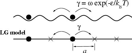
The driven LG model:

FK model: γ_± = w exp

æ
è

–ε ± aF

k_BT

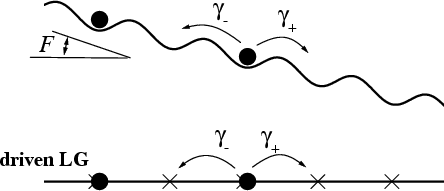
LG model: γ₊= γα and γ_–= γ(1–α), where 0.5 < α < 1; α≈aF/k_BT so that J ~ γ₊– γ_–

Underdamped system: two-state LG model

Underdamped system: inertia effects → bistability & hysteresis.

In the bistable region, two states: “immobile” and “running”. At jump, immobile → running

One-dimensional two-state LG model

Each atom may be either in an immobile state or in the running state

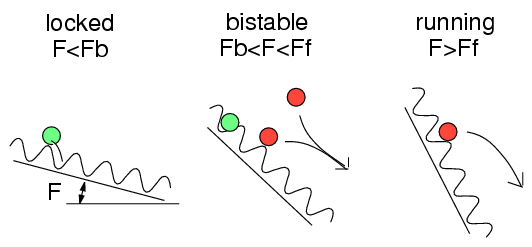
immobile (locked) state	running (sliding) state

rule: immobile → running (jump to empty state)	rule: running → immobile (collision with immobile atom)

Rules

1. At each time step t → t+1, one chooses at random a site i

2. If this site is occupied by immobile atom, it jumps to the site i+1

(if this site is empty) with the probability α,

or it jumps to the site i−1 (if the left-hand site is empty) with the probability 1−α.

After the jump to the left the atom remains in the immobile state,

while after the jump to the right the atom is in the running state.

3. If the atom in the chosen site i is in the running state,

it jumps to the right provided the right-hand site is empty,

and remains in the running state.

Otherwise, if the site i+1 is not empty, the atom in the site i remains in

the running state if the right-hand site is occupied by the running atom,

or becomes immobile if the site i+1 is occupied by the immobile atom.

4. Use periodic boundary conditions & sequential dynamics.

Note: open boundary condition → the partially asymmetric exclusion model

Evolution

The Frenkel-Kontorova model:

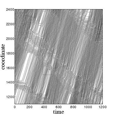
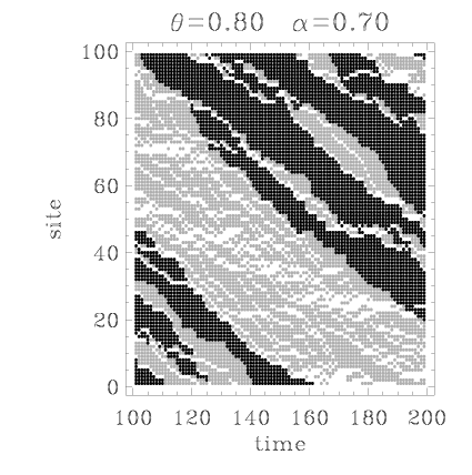
atomic trajectories versus time

Two-state lattice-gas model:

immobile atoms in black, running atoms in grey

Details of simulation for the FK model: we used Langevin motion equations,

x_i

+ η

x_i

+ sin x_i+

∂

∂x_i

[V(x_i+1–x_i) + V(x_i–x_i–1)] = F + δF_i(t)

with the exponential interatomic interaction, V(x)=V₀e^–βx, so that the elastic constant is g=V₀β²exp(–βa_A), and the parameters are a_A=a/θ, θ=2/3, g=0.1, T=0.1, η=0.1, β = 1/π, and f=0.33

The steady state

The LM-TJ model is solvable!

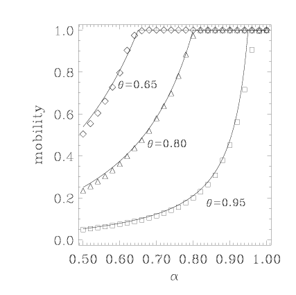
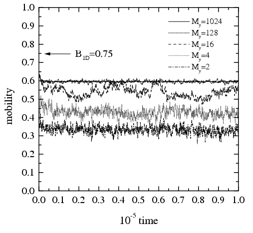
Let us define a dimensionless "mobility" B=N_r/N, where N_r is the number of running atoms. Then

B ≈

α(1–θ)

(1–α)θ

if α<θ

(*)

and B=1 for α>θ

Proof: Let there is only a sigle jam of the length s. Local concentration in the jam is θ_s=1, the length of the running domain (RD) is M_r. Then we maylet us use a simple arithmetic: s+N_r=N, s+M_r=M. Because N_r=M_rθ_r and N=Mθ, we have B=θ_r(1–θ)/(1–θ_r)θ. The most left site of any RD is always empty, therefore the running domain grows from its left-hand side with the rate α. The most right atom leaves the RD with the rate p_r, where p_r is the probability that the most right site of the RD is occupied. Approximately, p_r≈θ_r. Thus, we obtain the desired expression Eq.(*).

Kinetics of jams

Due to randomness of joining and losing events, the value s(t) exhibits random walks: at long times, t >>1, t^′ >>1, and |t–t^′| >>1, it behaves as ‹[s(t)–s(t^′)]²›≈2α|t–t^′|. Thus, at α < θ the infinite system has no steady state at all. A finite system does have a truly steady state corresponded to the absence of jams at all: Because the maximal jam's size is bounded, after a time τ, where ‹τ› = M²(θ–α)²/2α(1–α)², all jams disappear.

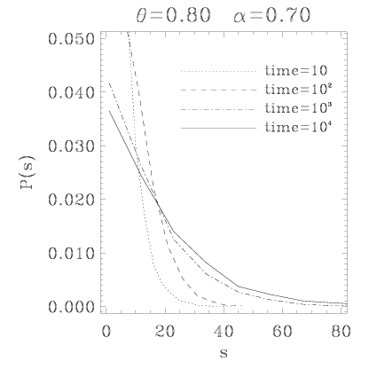
Distribution of jam's sizes: P(s) ~ exp(−s²/4αt) for s>>1 and t>>1

1D model vs 2D model ?

Conclusion for the 1D model: for θ>α there always exist traffic jams, B<1, due to: (a) randomness, and (b) hard-core interaction. The 1D model has no stationary state [although B(t)=const]. Thus, a receipts to avoid traffic jams are the following: (a) reduce θ, and (b) try to keep equidistance.

Question for a 2D model: B(2D) ↔ B(1D) ? Example: the two-lane model

concurrent processes:	{	(a)(a) detour TJs → B(2D) > B(1D)
		(b) creation of new TJs → B(2D) < B(1D)

Two-dimensional two-state LG model

Triangular lattice:

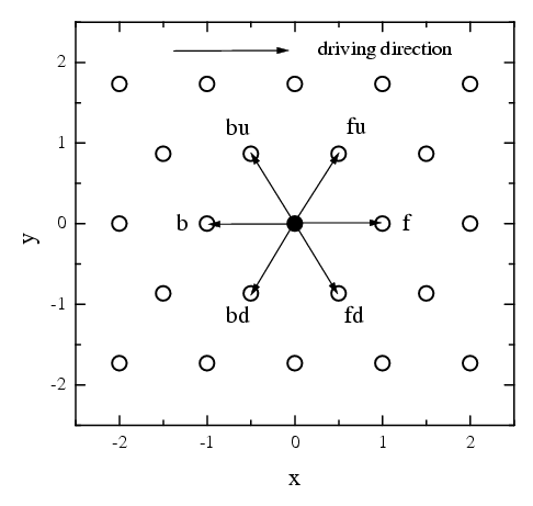f = forward

b = backward

u = up

d = down

Recall: γ_± = ω exp

æ
è

–ε ± aF

k_BT

ö
ø

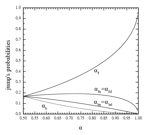
Use: α_f=α₀c², α_fu=α_fd=α₀c, α_b=α₀/c², α_bu=α_bd=α₀/c, where c~exp(aF/2T).

Normalization: α_f + α_fu+ α_fd + α_b + α_bu + α_bd = 1

Define: the total probability of the jump in the driving direction is α = α_f + α_fu + α_fd

Rules

1. Each atom may be either in an immobile state or in the running state.

2. At each time step t → t+1, one chooses at random a site i.

3. If this site is occupied by immobile atom, it jumps to one of six neighboring sites with

a corresponding probability, provided the chosen site is empty.

After the jump to one of three backward (left-hand side, i.e., b, bu, bd) directions

the atom remains in the immobile state, while

after the jump to the right (in the f-, fu-, or fd-direction)

the atom is in the running state.

4. If the atom in the chosen site i is in the running state, it jumps to the right

provided the right-hand site is empty, and remains in the running state.

Otherwise, if the right-hand site is not empty, the atom may either remain in the running state or it may

become immobile if the right-hand site is occupied by the immobile atom.

5. Use periodic boundary conditions & sequential dynamics.

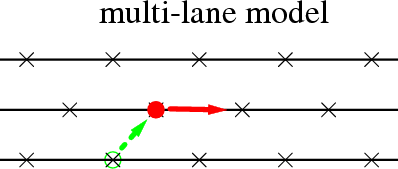
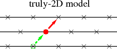
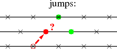
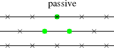
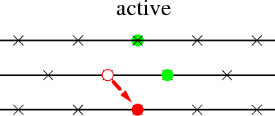
6. Four different variants: multilane model ↔ truly-2D model

passive jumps ↔ active jumps

Multi-lane and truly-2D models. The difference between multi-lane and truly-2D models is that in the multi-lane model, similarly to the 1D model, the running atom jumps to the right (in the f-direction) provided the site ahead of the running atom is empty, while in the truly-2D model the running atom remembers the direction of the previous jump (an analog of inertia effect in Newtonian dynamics) and continues to jump in the same direction (i.e., in the f-, fu-, or fd-direction). After the jump, the atom remains in the running state. If the site, to which the running atom has to jump, is occupied by a running atom, both atoms remain in the running state (in the truly-2D model we additionally assume that these two running atoms exchange by their jumping directions, similarly to momentum exchange in Newtonian dynamics). However, if the site, to which the running atom has to jump, is occupied by an immobile atom, the behavior is different for two more variants of the model:

Passive and active jumps. In the model with passive jumps, the running atom becomes immobile if the site, to which the running atom has to jump, is occupied by an immobile atom analogously to the 1D model. On the other hand, in the model with active jumps the running atom becomes immobile, only if all three sites (f, fu and fd) are occupied by immobile atoms. If one of these sites is empty, the running atom jumps to this site (in the case of two empty sites the jumping site is chosen randomly).

	/
	\

Evolution

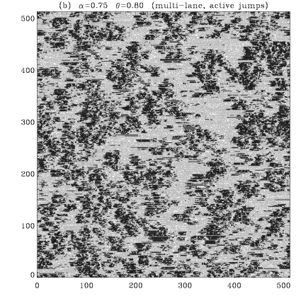
Example: multi-lane model with active jumps for α=0.75, θ=0.8 (see this figure enlarged)

snapshot: immobile atoms in black, running atoms in grey (lattice 512 x 512, t=10⁵)

Movies

short time scale (Δt=1) animated gif 3.3 Mb

long time scale (Δt=10) animated gif 5 Mb

both for multi-lane model with active jumps for α=0.75 and θ=0.8 (lattice 512x512, t_ini=10⁵)

immobile atoms in green, running atoms in red

2D model: distribution of jam sizes

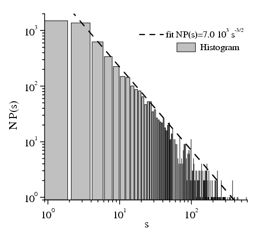
The 2D system has the truly steady state with a power law distribution of jam sizes characterized by the universal exponent 3/2: P(s) = As^–3/2, where A = ( ∑_s=1^∞ s^–3/2 )^–1 ≈0.383

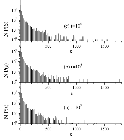Histogram of size distribution of immobile islands for the multi-lane model with active jumps at three times (t=10³, 10⁴ and 10⁵) for α=0.75, θ=0.8, M_x=M_y=1024 (enlarged view)

Histogram P(s) for the truly 2D model with active jumps (α=0.95, θ=0.8, M_x=M_y=512, t=10³, B≈0.64) (enlarged view)

Histograms for other parameters of the model are the following:

   multilane model with passive jumps:
      alpha=0.55, theta=0.50, file=lmpas-f.gif
      alpha=0.55, theta=0.70, file=lmpas-d.gif
      alpha=0.75, theta=0.70, file=lmpas-b.gif
      alpha=0.75, theta=0.80, file=lmpas-a.gif
      alpha=0.95, theta=0.88, file=lmpas-h.gif
   multilane model with active jumps:
      alpha=0.55, theta=0.50, file=lmact-f.gif
      alpha=0.75, theta=0.70, file=lmact-b.gif
      alpha=0.75, theta=0.80, file=lmact-a.gif
      alpha=0.95, theta=0.88, file=lmact-h.gif
      alpha=0.95, theta=0.90, file=lmact-e.gif
   truly 2D model with passive jumps:
      alpha=0.55, theta=0.50, file=2dpas-f.gif

      alpha=0.55, theta=0.70, file=2dpas-d.gif
      alpha=0.55, theta=0.90, file=2dpas-g.gif
      alpha=0.75, theta=0.60, file=2dpas-j.gif
      alpha=0.75, theta=0.70, file=2dpas-b.gif
      alpha=0.75, theta=0.80, file=2dpas-a.gif
      alpha=0.75, theta=0.90, file=2dpas-c.gif
      alpha=0.95, theta=0.70, file=2dpas-k.gif
      alpha=0.95, theta=0.80, file=2dpas-l.gif
      alpha=0.95, theta=0.88, file=2dpas-h.gif
      alpha=0.95, theta=0.90, file=2dpas-e.gif
      alpha=0.95, theta=0.94, file=2dpas-i.gif
   truly 2D model with active jumps:
      alpha=0.55, theta=0.62, file=2dact-m.gif
      alpha=0.55, theta=0.70, file=2dact-g.gif
      alpha=0.75, theta=0.70, file=2dact-b.gif
      alpha=0.75, theta=0.80, file=2dact-a.gif
      alpha=0.75, theta=0.90, file=2dact-c.gif
      alpha=0.95, theta=0.74, file=2dact-n.gif
      alpha=0.95, theta=0.80, file=2dact-l.gif
      alpha=0.95, theta=0.88, file=2dact-h.gif
      alpha=0.95, theta=0.90, file=2dact-e.gif
      alpha=0.95, theta=0.94, file=2dact-i.gif

Some analytical results

Consider the statistics of coalescence and splitting of immobile islands. Let

P_t(s) be the distribution of immobile islands at time moment t,

R(k+s, k) be the rate (per one time unit) of splitting of the island of size k+s into two smaller islands k and s, and

T(k+s, k) be the rate of coalescence of two islands k and s into one island of size k+s.

Master equation:

ΔP_t+1(s) ≡ P_t+1(s) – P_t(s) =

∞
∑
k=1

P_t(k+s) R(k+s,s) - P_t(s)

s–1
∑
k=1

R(s,k)

s–1
∑
k=1

T(s,k) P_t(k) P_t(s–k)

- P_t(s)

∞
∑
k=1

T(s+k,k) P_t(k).

The steady state must satisfy the equation ΔP_t(s)=0. Suppose that

(a) the rate of coalescence does not depend on the sizes of colliding islands, T(s, k)=T₀ for all s and k, and

(b) R(s, k) depends on the size of the island only, R(s, k)≈R(s).

In this case R(s) should behave as R(s) ~ (s–1)^–1 for s >> 1.

Proof: substituting T(s, k)=T₀ and R(s, k)=R(s) into the master equation for the steady state,

we can rewrite it in the form R(s) = [T₀a(s)+b(s)]/(s–1), where a(s)=–1+∑_k=1^s–1 P(k)P(s–k)/P(s) and b(s)=∑_k=s+1^∞ R(k)P(k)/P(s). Therefore, the splitting rate has to have the form R(s)=R₀/(s–1) for s>>1 provided the function a(s) has a finite limit, 0 < lim_s→∞ a(s) < ∞. However, such a limit exists only for the power-law distribution of island sizes, P(s)=ζ^–1(ν)s^–ν, where ζ(ν) is the Riemann zeta-function. Moreover, the function a_ν(s)=–1+ζ^–1(ν)s ^ν∑_k=1^s–1k ^–ν(s–k)^–ν has a nonzero limit for one value of the exponent ν only, namely ν≈3/2, as demonstrated in the figure below (see it enlarged).

Finally, the self-consistent solution of the steady state distribution is achieved with the parameters R₀ = CT₀, where C≈3 is the numerical constant.

Shape of jams

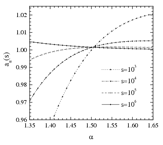
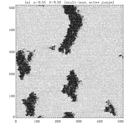
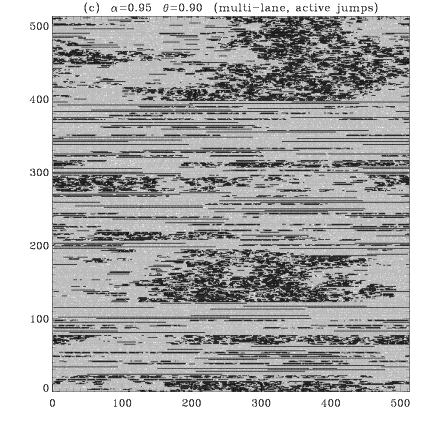
Snapshot configurations at t=10⁵ of the multi-lane model with active jumps (lattice 512 × 512) for different model parameters. Iimmobile atoms in black, running atoms in grey


(a) α = 0.55, θ = 0.5, B ≈ 0.8 (low forcing)	(c) α = 0.95, θ = 0.9, B ≈ 0.7 (high forcing)

Comparison of different models

Multi-lane vs truly-2D models and passive vs active jumps

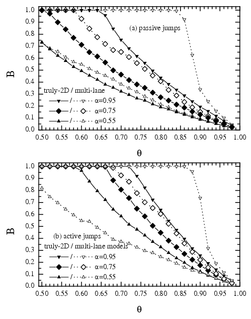
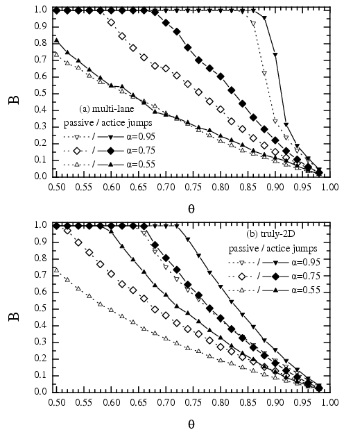
B(multi-lane) > B(truly 2D) in most cases, and B(active) > B(passive)


enlarged view	enlarged view

1D vs 2D models

In most cases B(1D) > B(2D):

Phase diagram

Conclusion

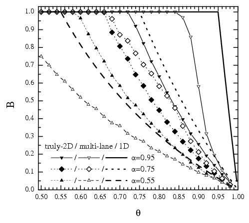
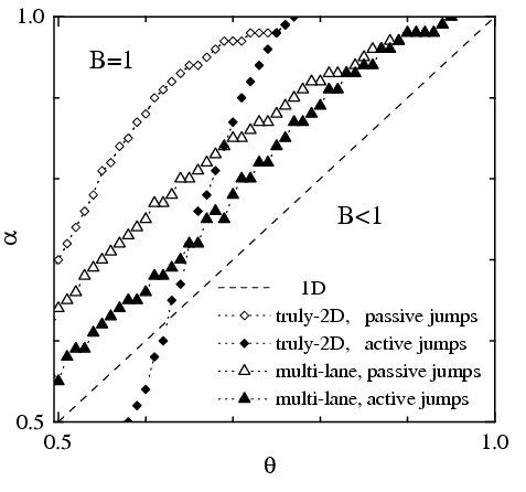
The 1D model: when θ > α, then the traffic jams exist always, B < 1, due to (a) randomness and (b) hard-core interaction. The 1D model has no stationary state (although B=const).

The 2D model has a truly steady state with a power-law distribution of jam sizes characterized by the universal exponent 3/2. Typically B(1D) > B(2D).

Receipts to avoid traffic jams:

(a) reduce the concentration θ;

(b) try to keep equidistance;

See Oleg Braun and Bambi Hu, J. Stat. Phys. 92 (1998) 629 "Traffic jams in a lattice-gas model" and Phys. Rev. E 71 (2005) 031111 "Two-dimensional two-state lattice-gas model" (pdf files may be found here)

Back to main page

Last updated on September 26, 2008 by Oleg Braun. Translated from L^AT_EX by T_TH